WaiDatathon 2021 - "Combat domestic violence with data and AI"
Detecting women at risk of domestic violence


WaiDatathon 2021: "Combat domestic violence with data and AI"

1. Problem description
The WaiDatathon 2021 was organized by Women in AI on the theme "Combat Domestic Violence with Data & AI". This notebook reproduces our main analysis for which we earned the first place at the competition.
Many professionals including social workers, medical professionals, academics, politicians or police agents are working daily to help women in abusive relationships, raise awareness in the general public and overall fight this phenomenon. Despite their efforts domestic violence is still a critical but hidden problem all around the world. When approaching this challenge it was clear for us that no amount of machine learning would solve the problem. Domestic violence is a sensitive and emotional topic for the victims. One of machine learning greatest strength is its ability to automate complex tasks, but domestic violence is a deeply human problem, and we believe that humans are the most important part of the support mechanism.
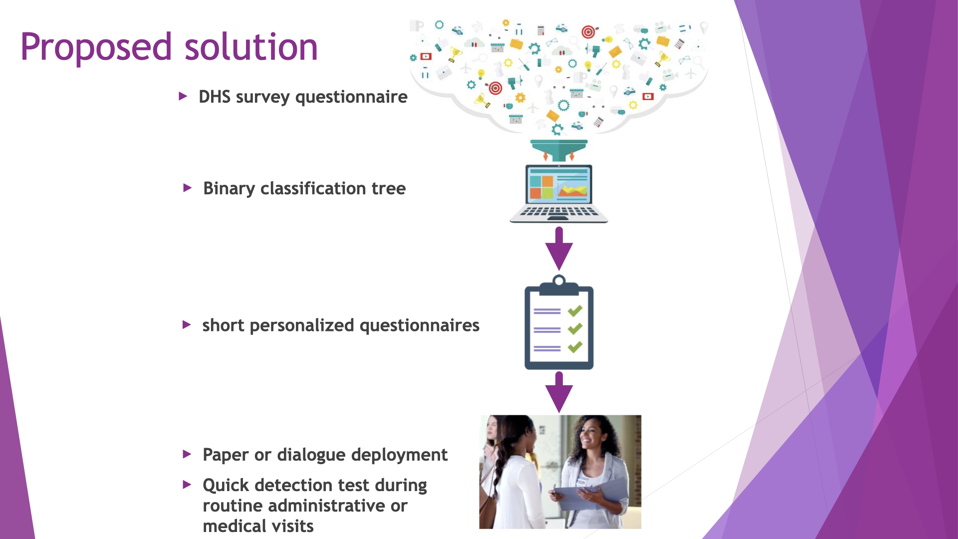
Three human parties are involved in domestic violence: the victim, the abuser and the supporters. We approached the challenge in two parts. Firstly, we addressed the victim's point of view. In particular, we tried to understand the relationships between the attitudes toward domestic and its occurence, and how these are affected by demographic characteristics. Secondly, we tried to provide an additional tools to supporters in order to detect women in danger. For this purpose we proposed a machine learning model that creates a questionnaire to detect early signs of domestic violence. Because the model can be deployed on paper or by dialogue, it is especially suited for developing countries.
You can watch our 5-minute competition talk here. The original notebook, data and presentation slides are available on the project's github repository.
1. Dataset description
Our analysis is based on the amazing data from The Demographic and Health Surveys (DHS) Program. This DHS program's goal is to collect, analyze and disseminate accurate and representative data on population, health, HIV and nutrition. It has run more than 400 surveys in 90 countries.
The dataset provided competition contains the results to the acceptability question (see below) aggregated per demographics (e.g. age, education, location). In other terms, this dataset contains information such as "70% of respondents with a secondary level of education answered 'yes' to a given question". However, since it does not contain the demographic information and answers of individual respondents it was not possible to cross mutliple information (e.g. age and education) or to build a predictive model.
To overcome this difficulty we obtained the complete DHS survey's women's questionnaire for Sub-Saharan countries. This dataset contains the response of individual respondents (samples) to thousands of questions (features). For a given country and a given survey phase the dataset would contain in the order of 10,000 samples and 4200 features. However, due to time constraints and the necessity to clean the data we did not use all the features but selected a subset of 38 questions.
For the competition we used data of the DHS survey for Benin and Congo, but to comply with copyright requirements of the DHS program only the example data of the DHS survey or generated by STATcompiler are contained in this github repository. Access to more data is free upon request on the DHS website. This notebook can be used to treat any survey data from the DHS women's questionnaire. However, since the survey questions are revised from one phase to another, some adjustements might be required in the data cleaning process when using earlier phases.
Some of the most important features for our analysis were in the form of multiple short questions on a given theme. We treated these questions either as:
- individual features
- a sum of positive answer (for a given theme)
- a boolean value (True if any question on a theme was answered true, False otherwise)
Below, we list these questions with their possible answers.
Important questions
Acceptability of violence:
Feature names: v744a - v744f
Possible answers:
- 0 No
- 1 Yes
- 8 Don't know
- (m) 9 Missing
- (na) Not applicable
In your opinion, is a husband justified in hitting or beating his wife when:
- she goes out without telling him?
- she neglects the children?
- she argues with him?
- she refuses to have sex with him?
marital control behaviors:
Feature name: d101a - d101e
Possible answers: see previous
Does your husband:
- become jealous or angry if you talks to other men?
- frequently accuses you of being unfaithful?
- not permit you to meet your female friends?
- tries to limit your contact with your family?
- insists on knowing where you are at all times?
- not trust you with money?
Physical violence:
Feature names: d105a - d105k
Possible answers:
- 0 Never
- 1 Often
- 2 Sometimes
- 3 Yes, but not in the last 12 months
- 4 Yes, but frequency in last 12 months missing
- (m) 9 Missing
- (na) Not applicable
Have you even been:
- pushed, shook or had something thrown by husband/partner?
- slapped by husband/partner?
- punched with fist or hit by something harmful by husband/partner?
- kicked or dragged by husband/partner?
- strangled or burnt by husband/partner?
- threatened with knife/gun or other weapon by husband/partner?
- physically forced into unwanted sex by husband/partner?
- forced into other unwanted sexual acts by husband/partner?
- had arm twisted or hair pulled by husband/partner?
- physically forced to perform sexual acts respondent didn't want to?
Emotional violence:
Feature names: d103a - d103c
Possible answers: see previous
Have you ever benn:
- humiliated by husband/partner?
- threatened with harm by husband/partner?
- insulted or made to feel bad by husband/partner?
# Import libraries
import matplotlib.pyplot as plt
import matplotlib as mpl
import pandas as pd
import numpy as np
import seaborn as sns
import plotly.express as px
import plotly.graph_objects as go
from IPython.display import HTML
# Customize figure output
plt.style.use('seaborn')
mpl.rc('font', size=18)
mpl.rc('axes', labelsize='large')
mpl.rc('xtick', labelsize='large')
mpl.rc('ytick', labelsize='large')
plt.rcParams['figure.figsize'] = [20, 10] # For larger plots
df = pd.read_csv('./Data/DHS_summary_world.csv', skiprows=1, skipfooter=11,engine='python')
df = df.merge(pd.read_csv('./Data/iso_alpha_list.csv'),
left_on='Country', right_on='country',how='left')
# Sample only the most recent survey for each country
country_list = df['Country'].unique().tolist()
temp = [df[df['Country']==country].reset_index().iloc[0] for country in country_list]
df = pd.DataFrame(temp).reset_index().drop(columns=['level_0','index'])
# Distributions
x = "Wife beating justified for at least one specific reason"
y = "Physical violence committed by husband/partner in last 12 months"
y_list = [x + " [Men]", x + " [Women]"]
temp = df[y_list].copy().rename(dict(zip(y_list,["Men", "Women"])),axis=1)
fig = px.violin(temp,box=True,title=x)
fig.update_layout(title=dict(x=0.5,font=dict(family='Futura')))
HTML(fig.to_html())
# Scatter plot of xperience vs acceptability of violence
from sklearn.linear_model import LinearRegression
# Data selection
x = "Wife beating justified for at least one specific reason"
y = "Physical violence committed by husband/partner in last 12 months"
colors = ['red','blue']
# Figure layout
fig = go.Figure(layout=dict(height=600,
xaxis=dict( title=x),
yaxis=dict( title=y),
legend=dict( title='country'),
title='Experience vs acceptability of violence'))
xlim = np.array([0,85])
ylim = np.array([0,50])
trace_flag = [] # flagging info for visualization: 0 for women, 1 for men, 2 for both
# Compute and plot regression lines
model = LinearRegression()
for i, gender in enumerate([" [Women]", " [Men]"]):
df_fit = df[[x + gender, y]].dropna()
X = df_fit[x + gender].values.reshape(-1, 1)
model.fit(X, df_fit[y])
x_range = xlim
y_range = model.predict(x_range.reshape(-1, 1))
fig.add_traces(go.Scatter(x=x_range, y=y_range,
name='Regression' + gender,
line=dict(color=colors[i],width=1),
marker=dict(opacity=0)),
)
trace_flag.append(i)
# Plot points for Women, Men and
for i in range(df.shape[0]): # loop over countries
fig.add_trace(go.Scatter(x=df[[x + " [Women]"]].iloc[i],
y=[df[y].iloc[i]],
marker=dict(color=['Red']),
line=dict(color='rgb(210,210,210)',width=1),
name=df['Country'].iloc[i],
))
trace_flag.append(0)
fig.add_trace(go.Scatter(x=df[[x + " [Men]"]].iloc[i],
y=[df[y].iloc[i]],
marker=dict(color='Blue'),
line=dict(color='rgb(210,210,210)',width=1),
name=df['Country'].iloc[i],
))
trace_flag.append(1)
# Plot a line that connects men and women for a given country
for i in range(df.shape[0]):
fig.add_trace(go.Scatter(x=df[[x + " [Men]", x + " [Women]"]].iloc[i],
y=[df[y].iloc[i],df[y].iloc[i]],
# color_discrete_sequence=['red'],
line=dict(color='rgb(210,210,210)',width=1),
marker=dict(size=0,color='black',opacity=0),
name=df['Country'].iloc[i],
))
trace_flag.append(2)
trace_flag = np.array(trace_flag)
# Update title, and axes range
fig.update_layout(title=dict(x=0.5,font=dict(family='Futura')))
fig.update_xaxes(range=xlim)
fig.update_yaxes(range=ylim)
# GUI
fig.update_layout(
updatemenus=[
dict(
type="buttons",
direction="right",
active=0,
xanchor='left',
x=0.01,
yanchor='top',
y=0.98,
buttons=list([
dict(label="Women and Men",
method="restyle",
args = [{'visible': np.ones(len(trace_flag))}],
),
dict(label="Women only",
method="restyle",
args = [{'visible': trace_flag==0}]
),
dict(label="Men only",
method="restyle",
args=[{'visible': trace_flag==1}]),
])
)
]
)
HTML(fig.to_html())
There seems to be a certain correlation between acceptability and experience of violence although the data are quite scattered. The regression line tells us that on average, for every 10% acceptability, domestic violence increases by ~2% (women acceptability) and 4% (men acceptability). In most countries the acceptability score is much higher than the experience score which indicates either that even woman who don't experience domestic violence find it acceptable or that domestic violence is largely unreported.
# create figure
acc = "Wife beating justified for at least one specific reason" + " [Women]"
exp = "Physical violence committed by husband/partner in last 12 months"
fig = go.Figure(layout=dict(width=700,height=550))
hover_text = 'country: ' + df['country'] + "<br>" + \
'experience: ' + df[exp].astype(str) + ' %<br>' + \
'acceptability: ' + df[acc].astype(str) + ' %<br>'
# Add surface trace
fig.add_trace(go.Choropleth(z=(df[acc]-df[exp])/df[acc].values.tolist(),
locations=df['iso_code'].values.tolist(),
text=hover_text, hoverinfosrc='text',
visible=False,
zmin=-1.0,
zmax=1.0,
colorscale='PiYG_r',
colorbar=dict(title=dict(text='(acc-exp)/acc []',side='right'))
))
fig.add_trace(go.Choropleth(z=df[exp].values.tolist(),
locations=df['iso_code'].values.tolist(),
text=hover_text, hoverinfosrc='text',
colorscale="Greens",
visible=False,
colorbar=dict(title=dict(text='experience [%]',side='right'))
))
fig.add_trace(go.Choropleth(z=df[acc].values.tolist(),
locations=df['iso_code'].values.tolist(),
text=hover_text, hoverinfosrc='text',
colorscale="Reds",
colorbar=dict(title=dict(text='acceptability [%]',side='right'))
))
fig.update_layout(title=dict(x=0.5,
text='World distribution of acceptability and experience of domestic violence',
font=dict(family='Futura')))
fig.update_layout(
updatemenus=[
dict(
type="buttons",
direction="right",
active=0,
xanchor='center',
yanchor='bottom',
x=0.5,
y=1.02,
buttons=list([
dict(label="Acceptability",
method="restyle",
args = [{'visible': [False, False, True]}]
),
dict(label="Experience",
method="restyle",
args=[{'visible': [False, True, False]}]),
dict(label="(Acceptatbility-Experience)/Acceptability",
method="restyle",
args = [{'visible': [True, False, False]}]),
]),
showactive=True,)
])
HTML(fig.to_html())
The above figure shows the distribution of acceptability and experience of violence among women. Here, violence is considered as "acceptable" for the respondent if she answered any of the acceptability question positively. Here, the experience of violence corresponds to any positive answer (answer other than "never") to any of the physical violence question. The dataset was generated using STATcompiler.
Acceptability is calculated as the percentage of women who answered "True" to at least one of the acceptability question. While experience counts the percentage of women who answer "yes, in the last twelve" to at least one of the physical violence question. The (normalized) difference map is computed as $(acceptability-experience)/acceptability$.
Both acceptability and experience are highest in Afghanistan. Acceptability is highest in subsaharan african countries, middle east and south/southeast Asia, and lowest in Europe and Latin America. Experience is above 10% in most countries and highest in Papua New Guinea and Afghanistan. The difference map shows, in green, countries where acceptability is lower experience than experience. This situation may be seen as a good thing if we consider that public awareness may drive a change in society as suggested by the fact that these countries have relatively lower experience percentage points. In countries colored purple experience is higher than acceptability. These countries tend to have relatively high experience scores. Angola has a score close to 0, due to a relatively low acceptability but high experience. Could this low acceptability score signal that a change is about to come in Angola?
The numbers shown here, and especially the experience score must be taken as lower bounds since domestic violence is most likely under-reported.
First, we load the DHS women questionnaire model dataset.
# Load data
df_IR = pd.read_stata("./Data/ZZIR62FL.DTA", convert_categoricals=False)
print(f"Number of samples: {df_IR.shape[0]}")
print(f"Number of features: {df_IR.shape[1]}")
Then, we manually select a subset of features. We store the code of each feature in variable with a more explicit name.
# Subset of features
# background
edu = 'v106' # education
violence_justified = 'v744' # a-e
age = 'v012'
age_group = 'v013'
litteracy = 'v155'
media_paper = 'v157'
media_radio = 'v158'
media_tv = 'v159'
sample_weight = 'v005' # must be divided by 1e6
ever_married = 'v020'
# residence = 'v025'
time2water = 'v115'
has_elec = 'v119'
has_radio = 'v120'
has_tv = 'v121'
has_fridge='v122'
has_bicycle = 'v123'
has_moto = 'v124'
has_car = 'v125'
religion = 'v130'
ethnicity = 'v131'
place_of_residence = 'v134'
edu_attainment = 'v149'
relation2household_head='v150'
sex_household_head = 'v151'
age_household_head = 'v152'
has_phone_landline='v153'
has_phone_mobile='v169a'
use_internet = 'v171a'
use_internet_last_month = 'v171b'
wealth_index = 'v191'
total_child_born = 'v201'
num_sons_died = 'v206'
num_daughters_died = 'v207'
num_dead_child = 'num_dead_child'
num_living_child = 'v218'
husband_edu_level = 'v701'# 's904'
husband_occupation = 's908a'
resp_occupation = 's913a'
# Domestic violence
selected_for_dom_violence_interview = 'v044'
is_currently_in_union= 'v502'
weight_dom_violence = 'd005'
control_issues = 'd101' #a-j
num_control_issues = 'd102'
emotional_violence = "d103" # a-f
emotional_violence_any = 'emotional_violence_any' #'d104'
physical_violence = 'd105' # a-n detailed acts of violence
physical_violence_less_severe = 'd106'
physical_violence_severe = 'd107'
sexual_violence = 'd108'
violence = 'violence'
# any_violence = 'd105' or 'd106' or 'd107'
violence_to_husband ='d112'
partner_drinks_alcohol='d113'
partner_drinks_alcohol_freq = 'd114'
sought_help = 'd119' # a to xk; y=no one
mother_beaten = 'd121'
edu_w = 'v106' # education level women, value =0-3
edu_m = 'mv106' # education level men,
#Age (v012) is recorded in
#completed years, and is typically reported in 5-year groups (v013).
# age_group_w = "v013"
# Info for men is in the Men's individual recode (MR) dataset
list_col0 = ['caseid', 'v000', sample_weight,
edu, age, age_group, litteracy,
media_paper, media_radio, media_tv,
ever_married,
has_elec, has_radio, has_tv, has_fridge, has_bicycle, has_car, has_moto,
has_phone_landline,
# has_phone_mobile,
religion, ethnicity,
place_of_residence, age_household_head,
relation2household_head,
wealth_index,
total_child_born, num_living_child,
husband_edu_level,
# husband_occupation, resp_occupation,
selected_for_dom_violence_interview, weight_dom_violence,
is_currently_in_union, num_control_issues, #emotional_violence_any,
physical_violence_less_severe, physical_violence_severe, sexual_violence,
partner_drinks_alcohol, partner_drinks_alcohol_freq, #sought_help,
mother_beaten
]
print(f"Number of feature selected: {len(list_col0)}")
2. Data cleaning
First we clean the data for our "important questions" (see intro). We encode these questions using one-hot encoding (True or False). And create new features as the sum of answers on a given topic. We will treat missing values (code 9) as False. We will consider True answers "Yes", "Often", or "Sometimes". All other answer are consider false. The details of the possible answers are given in the next cell. NA values will be dealt with a a few cells later.
# Prepare clean format for multiple questions
# Violence_justified
# =======
'''
V744A Beating justified if wife goes out without tell 6103 1 N I 1 0 No No
0 No
1 Yes
8 Don't know
(m) 9 Missing
(na) Not applicable
'''
# I assume 0 if v744 in [0, 8, 9, na]; 1 otherwise
# Control issues
# =======
'''
D101A Husband/partner jealous if respondent talks wit 8272 1 N I 1 0 No No
0 No
1 Yes
8 Don't know
(m) 9 Missing
(na) Not applicable
'''
# For cleaning: same as previous
# Physical or sexual violence
# =======
'''
D105A Ever been pushed, shook or had something thrown 8291 1 N I 1 0 No No
0 Never
1 Often
2 Sometimes
3 Yes, but not in the last 12 months
4 Yes, but frequency in last 12 months missing
(m) 9 Missing
(na) Not applicable
'''
# Let's consider true if hit during the past 12 months only
# So, we clean as 0 if d105a in [0, 3,4,9,na]
# Emotional violence
# =======
'''
D103A Ever been humiliated by husband/partner 8284 1 N I 1 0 No No
0 Never
1 Often
2 Sometimes
3 Yes, but not in the last 12 months
4 Yes, but frequency in last 12 months missing
(m) 9 Missing
(na) Not applicable
'''
# Same as physicial violence for cleaning
cleaning_dict = {
violence_justified: {'ind': 'abcde', 'values_0': [8,9], 'values_1': [1]},
control_issues: {'ind': 'abcdefghij', 'values_0': [8,9], 'values_1': [1]},
physical_violence: {'ind': 'abcdefhijk', 'values_0': [3,4,9], 'values_1': [1,2]}, # ind: g skipped intentionally (NA)
emotional_violence: {'ind': 'abc', 'values_0': [3,4,9], 'values_1': [1,2]}
}
# Add multiple questions to list_col
list_col = list_col0.copy()
for key in cleaning_dict.keys():
cleaning_dict[key]['list_col'] = [key + letter for letter in cleaning_dict[key]['ind']]
list_col += cleaning_dict[key]['list_col']
Next we create a new dataframe that contains data only for the women who answered the domestic violence questionnaire. This will deal with the NA values. Then, we create the new xxx_sum features
# Create a subset dataframe that contains only the chosen columns
# and only for women who are married and took the domestic violence interview
df = df_IR[list_col].copy()
df = df[df[is_currently_in_union]==1]
df = df[df[selected_for_dom_violence_interview]==1]
print(f"Number of samples: {df.shape[0]}")
print(f"Number of features: {df.shape[1]}")
for key in cleaning_dict.keys():
df[key + '_sum'] = 0
for letter in cleaning_dict[key]['ind']:
df[key + letter].fillna(0, inplace=True) # There shouldn't be missing na because of preselection of samples, but just in case
for i in cleaning_dict[key]['values_0']:
df.loc[df[key + letter] == i,key + letter] = 0
for i in cleaning_dict[key]['values_1']:
df.loc[df[key + letter] == i,key + letter] = 1
df[key + '_sum'] += df[key + letter]
# Check that assignment is correct
assert df[key + letter].max() <= 1
# print(key + letter + ":", df[key + letter].max())
temp = df[[violence_justified + '_sum', physical_violence + '_sum']].copy()
temp['value'] = 1
temp.loc[temp[physical_violence + '_sum']>=1, physical_violence + '_sum']=1
temp.loc[temp[violence_justified + '_sum']>=1, violence_justified + '_sum']=1
temp_pivot = temp.pivot_table(columns=[physical_violence + '_sum'],
index=[violence_justified + '_sum'],
values='value',aggfunc='count')
display(temp_pivot)
# fig, ax = plt.subplots(3,1,figsize=[8,8],gridspec_kw={'hspace':0.5})
plt.sca(ax[0])
plt.title('Number of respondents for each class of score (only respondent not experience domestic violence)',fontsize=18)
sns.barplot(x=temp_pivot.index, y=temp_pivot.loc[:,0])
plt.xticks([])
plt.xlabel('')
plt.ylabel('')
plt.sca(ax[1])
plt.title('% of respondents experiencing domestic violence for each class',fontsize=18)
sns.barplot(x=temp_pivot.index, y=temp_pivot.loc[:,1]/temp_pivot.loc[:,0]*100,ax=ax[1])
plt.xlabel('')
plt.ylabel('')
plt.xticks([])
plt.sca(ax[2])
plt.title('Number of respondents for each class of score (only respondent experiencing domestic violence)',fontsize=18)
sns.barplot(x=temp_pivot.index, y=temp_pivot.loc[:,1])
plt.ylabel('')
_ = plt.xlabel('class')

- subplot(1) most respondents answered no to every question (ie v744_sum == 0)
- subplot(2) Given the v744 score, the probability to experience violence is higher for higher scores (i.e., P(A|B), where A is score and B is violence)
- subplot(3) since there are many more people with a score of 0, most people experiencing violence scored 0 (i.e. P(B|A))
The results from subplot 2 and 3, are typical examples of bayesian probability.
key = physical_violence
physical_violence_questions_sum = df[[key + letter for letter in cleaning_dict[key]['ind']]].sum()
num_physical_violence_respondent = (df[physical_violence + '_sum']>0).sum()
question_list = [
"pushed, shook or had something thrown at",
"slapped",
"punched with fist or hit by something harmful",
"kicked or dragged",
"strangled or burnt",
"threatened with knife/gun or other weapon",
"physically forced into unwanted sex",
"forced into other unwanted sexual acts",
"had arm twisted or hair pulled",
"physically forced to perform sexual acts",
]
physical_violence_questions_sum.rename(dict(zip(physical_violence_questions_sum.index, question_list)),inplace=True)
physical_violence_questions_sum.sort_values(ascending=False,inplace=True)
_ = sns.barplot(x=physical_violence_questions_sum/num_physical_violence_respondent*100, y=physical_violence_questions_sum.index,orient='h')
_ = plt.xlabel('% of respondents')

phys_less = df[['d105a', 'd105b', 'd105c', 'd105j']].copy()
phys_more = df[['d105d', 'd105e', 'd105f']].copy()
sexual = df[['d105h', 'd105i', 'd105k']].copy()
emo = df[['d103a', 'd103b', 'd103c']].copy()
names = ["emo", "phys_less", "phys_more", "sexual"]
temp_dict = {}
for name, this_df in zip(names, [emo, phys_less, phys_more, sexual]):
temp_dict[name] = (this_df.sum(axis=1)>0).astype(float)
# this_df
temp = pd.DataFrame(temp_dict)
co_occurence = (temp.T@temp)#.astype(float)#.values
for i in range(co_occurence.shape[0]):
co_occurence.iloc[i,:] /= co_occurence.iloc[i,i]
temp.head()
temp['any'] = (temp.sum(axis=1)>0).astype(float)
proba = temp.sum()/temp.shape[0]
proba
# co_occurence.head()
# co_occurence = np.concatenate([ , co_occurence],axis=0)
fig, ax = plt.subplots(1,2,figsize=(20,6))
plt.sca(ax[0])
sns.barplot(x=proba.index, y=proba)
_ = plt.title("Probability event individual events",fontdict={'fontsize':20})
plt.sca(ax[1])
co_occurence.style.background_gradient(cmap='magma', low=0.0, high=0.,axis=1)
sns.heatmap(co_occurence*100,annot=True)
ax = plt.gca()
# ax.xaxis.grid(True, which='major')
ax.set_yticklabels(co_occurence.index,fontdict={
'verticalalignment': 'center',}
)
_ = plt.title("Probability event A (column) given (event) B (row), i.e. P(A|B)",fontdict={'fontsize':20})
xx, yy = np.meshgrid(np.arange(15),np.arange(15))
_ = plt.plot(xx.T,yy.T,'w',lw=15)

The above graph summarizes the forms of violence experienced by women in the last 12 months. Those results are for the model dataset and for the women who answered to the domestic violence questionnaire. The left graph shows that out of the respondents 21% experienced emotional violence, ~27% "less severe" physical violence, ~12% severe physical violence, ~4% sexual violence, and ~30% experience at least one of these kind of violence. The right graph shows the probability that a woman who experiences a form of violence B (row) also experiences the form of violence A. For example, the first row shows that woman who experience emotional violence also expereince less severe physical violence at 71%, severe physical violence at 34% and sexual violence at 12%. Here, we see that emotional violence is rarely isolated: more than 2/3 of women experiencing emotional violence also experience some form of physical violence. Overall experiencing emotional violence raises the likelihood of other acts of violence roughly by a factor of 3. For example, 4% of women from the general population experience sexual, while 12% of those who experience emotional violence do. However, emotional violence is not always experienced by women in abusive relationship: only 64% of women experiencing severe physical violence also experience emotional violence. It is a surprisingly low number compare to the 89% of women in that situation who also experience less severe violence.
In this section we will attempt to predict which women is experiencing physical or sexual domestic violence based on their other answers to the DHS women questionnaire. More precisely, we will attempt to predict for any given woman, her answer ("yes" or "no") to the question "Have you experienced any form of physical or sexual domestic violence in the last 12 months?". In the following sections We quantify the predictivity of features based on the mutual information score and we build use a decision tree algorithm to build a very short personalized questionnaire whose goal is to identify women at risk of domestic violence.
# Select some features for mutual information analysis
list_col_model = [
litteracy,
age,
mother_beaten,
wealth_index,
num_living_child,
edu,
husband_edu_level,
partner_drinks_alcohol_freq,
control_issues + '_sum',
violence_justified + '_sum',
emotional_violence + '_sum',
physical_violence + '_sum',
]
X = df[list_col_model].copy()
explicit_feature_names = [
'Literacy',
'Age',
'Did your mother ever experience domestic violence?',
'wealth index',
'number of children',
'Education level',
"Husband's education level",
'How often does your husband drink alcohol?',
'Is your husband jealous, or not trusting you with money?',
'Is a husband justified to beat his wife?',
'Have you ever been humiliated, insulted or threatened by your husband?',
]
# replace not applicable by "doesn't drink" for alcohol related question
for col in [partner_drinks_alcohol_freq, mother_beaten]:
X[col].fillna(0, inplace=True)
# feature engineering
age_diff = 'age_diff'
age_ratio = 'age_ratio'
X.loc[:,'v701'].fillna(0,inplace=True) # only 2 missing values in Congo, 0 in Benin
X.loc[X[litteracy]>=3,litteracy] = 0
X.loc[X[litteracy]<=1,litteracy] = 0
X.loc[X[litteracy]==2,litteracy] = 1
# cast the following columns as int8 to treat them as discrete features
for col in [ partner_drinks_alcohol_freq, mother_beaten,
husband_edu_level]:
X.loc[:,col] = X.loc[:,col].astype('int8') # /!\ contains "8" as Nan
# cast the following columns a floats continuous features
for col in [num_living_child, #num_dead_child, total_child_born,
age, #age_household_head, age_diff,
violence_justified + '_sum',
emotional_violence + '_sum',
physical_violence + '_sum',
control_issues + '_sum',
wealth_index]:
X[col] = X[col].astype(float)
discrete_features = X.dtypes == 'int8'
X.dropna(inplace=True)
# Mutual information classification
from sklearn.feature_selection import mutual_info_classif
def make_mi_scores(X, y, discrete_features):
mi_scores = mutual_info_classif(X, y, discrete_features=discrete_features)
mi_scores = pd.Series(mi_scores, name="MI Scores", index=X.columns)
mi_scores = mi_scores.sort_values(ascending=False)
return mi_scores
def plot_mi_scores(scores):
scores = scores.sort_values(ascending=True)
width = np.arange(len(scores))
ticks = list(scores.index)
plt.barh(width, scores)
plt.yticks(width, ticks)
plt.title("Mutual Information Scores", fontsize=25)
# Let's try subsampling the majority class (no violence) to get better classification on the minority class (i.e. the class of interest)
from sklearn.model_selection import train_test_split
def subsample(X,y,imbalance_fac=1):
y_select = df[physical_violence + "_sum"]>0
y_negative = y[y_select==0].copy()
y_positive = y[y_select==1].copy()
X_negative = X.loc[y_select==0,:].copy()
X_positive = X.loc[y_select==1,:].copy()
_, X_negative_sub, _, y_negative_sub = train_test_split(X_negative,y_negative, test_size=imbalance_fac*len(y_positive))#, stratify=True )
return (pd.DataFrame(np.concatenate([X_negative_sub,X_positive]), columns=X.columns),
pd.Series(np.concatenate([y_negative_sub,y_positive]), ))
for itarget, target_feature in enumerate([physical_violence]):
y = X[target_feature + '_sum']>0
plt.subplot(1,2,itarget+1)
this_X = X.drop(columns=[target_feature + "_sum"] )
discrete_features = this_X.dtypes == 'int8'
mi_scores = pd.Series(np.zeros(this_X.columns.shape), index= this_X.columns)
n = 20
for i in range(n):
X_sub, y_sub = subsample(this_X,y)
mi_scores += 1.0/n*make_mi_scores(X_sub, y_sub, discrete_features)
mi_scores.rename(dict(zip(X.columns,explicit_feature_names)), inplace=True)
plot_mi_scores(mi_scores)

The above bar graph shows the mutual information of the features selected for modeling. Mutual information measures how much information about our target value is gained by knowing the information related to the given feature. Here our target value is any positive answers to the question set about domestic physical or sexual violence, where a positive answer correspond to answers "Often" or "Sometimes". We summarize the target question as: "Have you experienced any form of physical or sexual domestic violence in the last 12 months?". By far the most predictive feature is the sum of answers to the question about emotional violence, which we summarize as "Have you ever been humiliated, insulted or threatened by your husband?". We explored in detail the relation between emotional and physical/sexual violence in the "exploratory data analysis" section. The second most predictive feature is the sum of positive answers to the question set about controlling behavior of the husband. Then, come several demographic information such as age, wealth index, number of children, education, litteracy. We see that the acceptability of violence ("Is a husband justified to beat his wife?") has much less predictivity than emotional violence or husband's controlling issues. However, it is slightly more predictive than husband's drinking habits.
3. Model training
Finally, we use the sklearn library's binary classification tree to create a model that predicts whether a woman has been experiencing deomestic violence in the last twelve month based on the set of features that we selected. A binary classification tree iteratively divides the features space in halves. At each stage the division of the space is chosen so that each new subdomain (or leaf) becomes "purer". A "pure" leaf would only contain women experiencing domestic or only women not experiencing violence. A leaf where half in which half of the women experience violence and the other not would be "unpure".
In our case, the "True" class corresponds to women already domestic violence. That means that the model's result can be divided as follows:
- True positive ($TP$): women already experiencing domestic violence and correctly classified by the model
- True negative ($TN$): women not experiencing domestic violence and correctly classified
- False positive ($FP$): women not experiencing domestic violence but classified as "experiencing violence" by the model
- False negative ($FN$): women experiencing domestic violence but not detected by the model
Here, false negative are women already in danger but not deteced. Thus, the first priority of the model would be to limit false negatives. False positive may correspond to women who, although they are not experiencing domestic violence, may be in a situation where other forms of abusive are taking place such as emotional violence or controlling behaviors. For practical purpose interviewees classified as True positive or False positive should both be offered additional help.
Choice of performance metric
We need a metric to evaluate the model's performance and optimize the hyperparameters. We need to evaluate possible metrics based on the specific goals of our model. Typical metrics are:
- accuracy: $\frac{TP+TN}{TP+FP+FN+TN}$
- F1-score: $\frac{2*TP}{2*TP+FP+FN}$
- precision: $\frac{TP}{TP+FP}$
- recall: $\frac{TP}{TP+FN}$
- negative predictive value: $\frac{TN}{TN+FN}$
In classification task, the most often used metric are accuracy and F1-score. However, both metrics as well as precision would tend to limit $FP$ which is against our objective. Since our primary objective is to limit the $FN$ "recall" and "negative predictive value" are the most adequate metrics. We chose recall because it would maximize $TP$, which is more interesting than $TN$ in our case.
Choice of hyperparameters to optimize
We optimize the minimum of samples per leaf. This parameter also implicitly controls the depth of the tree. For our purpose, we do not need the most accurate model possible since we keep a human in the loop. In practice, the model would be used by an interviewer as a tool to direct the early stages of an interview and form his opinion on whether the woman interviewed should be proposed specific help. In this sense the model prediction would probably be used in a qualitative rather than quantitative way.
from sklearn.tree import DecisionTreeClassifier
from sklearn. ensemble import GradientBoostingClassifier, RandomForestClassifier
from sklearn.model_selection import train_test_split
from sklearn.metrics import accuracy_score
from sklearn import tree
from sklearn.metrics import confusion_matrix, classification_report
from sklearn.model_selection import GridSearchCV
from sklearn.metrics import f1_score, roc_auc_score
y = X[physical_violence + "_sum"]>0
this_X = X.drop(columns=[physical_violence + "_sum"])
this_X = this_X.rename(dict(zip(this_X.columns,explicit_feature_names)),axis=1)
discrete_features = this_X.dtypes == 'int8'
X_model = pd.get_dummies(this_X, columns=this_X.columns[discrete_features])
imbalance_fac = 1
X_model, y = subsample(X_model,y, imbalance_fac=imbalance_fac)
X_train, X_test, y_train, y_test = train_test_split(X_model.values,y.values, test_size=0.2)
param_grid = dict(max_depth=[9],
min_samples_leaf=[0.01, 0.02, 0.03, 0.05, 0.07, 0.1, 0.15, 0.2],
)
clf = DecisionTreeClassifier(min_impurity_decrease=0.0001,
class_weight={0:1, 1:imbalance_fac},
)
clf_cv = GridSearchCV(clf, param_grid, cv=3, scoring='recall')
clf_cv.fit(X_train, y_train)
display(clf_cv.best_params_)
y_pred = clf_cv.best_estimator_.predict(X_test)
print(confusion_matrix(y_test, y_pred)/y_test.shape[0])
classif_dict = classification_report(y_test,y_pred, output_dict=True)
print("f1_score:", classif_dict['True']['f1-score'])
print(classification_report(y_test,y_pred))
Here, the optimal parameter was minimum number of samples per leaf (min_samples_leaf) of 0.05.
The model achieved a recall of 63% for the True class and a F1-score of 70% fo both classes. Next, we visualize the model results to get a better sense of the quality of the classification.
_ = tree.plot_tree(clf_cv.best_estimator_, feature_names=X_model.columns, filled=True,
impurity=False, proportion=True, precision=2, rounded=True,fontsize=12)

Because all our features correspond to questions asked during the DHS questionnaire, each branching of the tree corresponds to question, and each branch to an answer. Unlike other machine learning algorithms, a decision tree can work with partial data. Firstly, because the tree doesn't use every single feature of the dataset to build a prediction. Secondly, because you only need the answers relative to path you are taking down the tree. Therefore, the model can be used to interview women. The interviewer would first ask the question at the root of the tree, and then ask the next relevant question depending on the answer given.
For example, the first question would be to ask the questions related to emotional violence (see introduction), which can be summarized as "have you ever been humiliated, insulted or threatened by your husband?". If the interviewee answers "yes", then the model predict that there is 89% chance that she experiences domestic violence, so she should be proposed further help. If she answers "no", the next question would be to ask if there is a history of violence in her family, etc...
5. Discussion
As we mentionned earlier, classically the value of a model is to provide an accurate prediction. However, in our case the value of the model resides in:
- The graph shown above which is the main tool: it allows an interviewer to direct an interview in the most efficient way possible.
- The prediction. At each node of the model, the proportion of negative and positive class can be viewed as the probability that the interviewed woman needs further help. These predictions are probably more useful in a qualitative or a rough quantitative way. For example the probability can be divided into three buckets:
- $<30$% positive (orange) this woman doesn't need help
- $30-70$% (white): this woman may need help
- $>70$%: this woman needs help
Here, we used arbitrary limits of 30% and 70%, but in practice, these limits would be place by the interviewer or relevant organism depending their on objectives, budget, availability of helpers etc... And of course this short questionnaire can be just a small part of a longer interview.
We chose a decision tree as a model because it is transparent (i.e. white-box model) and can be used by humans using the output flow chart. However, decision trees have the inconvenient of not being robust. That means that slight changes in the data can result in a significantly different tree. In our experience, the root of the tree is very robust and never changes. The first level is also relatively robust. Beyond this level, different branches may occur. This points out to the fact that within random variations of the dataset many "good" questionnaires are possible, in the same way that a human interviewer would not ask always the same questions. Thus, we emphasize again that the decision tree constitutes a good tool to guide the decision process of a human interviewer.
However, the questions we identified are related to emotional violence and control issues. These are sensitive topic, and these questions may be perceived as intrusive. In that case, the interviewee may become uncomfortable or lie. Therefore, for practical purposes it might be beneficial to train the model with less informative but less intrusive questions such as demographics information. Both questionnaire could even be used together. First, the less intrusive questionnaire would be used for a first screening. The interviewee scoring above a predefined probably could then be asked questions from the more informative but more intrusive questionnaire, possibly by another person or in a more comfortable context.
Domestic violence is still an unsolved problem in 2021. The data from the Demographics and Health Survey reveal that in developing countries, a signifificant proportion of women (5-50%) report having experienced domestic violence in the last twelve months. Furthermore, on average, 35% of women think that this violence is justified.
In this report, we presented an extended version of our contribution to the Women in AI Datathon 2021 on the theme "combat domestic violence with data and AI". Our analysis is based on statistics compiled using the DHS' STATcompiler and our own analysis of the sample questionnaire. We note that results based on this sample dataset are consistent with the results for Congo and Benin that we presented at the competition.
We attempted to identify the most relevant questions from the DHS survey questionnaire to identify women in a situation of domestic violence or at risk of domestic violence. We found that the most informative questions were the ones related to emotional violence and control issues. The wealth index is the most informative demographics information, although it scores 6 times less than emotional violence on the mutual information score.
Since domestic is a sensitive and emotional topic for the women experiencing it, we believe that human contact with helpers is of primary importance. Therefore we designed our AI system not with the goal of automating a task, but to provide a tool to inform and assist helpers. This tool comes in the form of a personalized questionnaire generated using a classification tree algorithm. This questionnaire can be used by health or social professionals to efficiently carry out quick interview and form a rapid opinion on whether the interviewed woman is at risk of domestic violence and should be provided with further help. Although we found that the most informative questions are related to emotional violence and control issues, those may be very sensitive issues. For the purpose of short interviews the model could be improved by training in on less intrusive questions, even if those questions are less informative.